Benchmark: Interactions between Convolution and Pooling layers in Graph Neural Networks
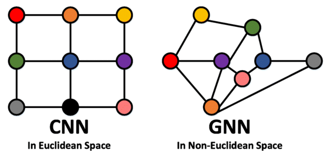
Why Considering Graphs?
Source: Lin et al., 2021
\(\hookrightarrow\) GNN can be seen as an extension of CNN to any topology.
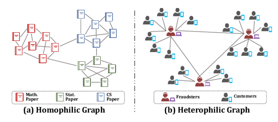
The Notion of Homophily
Source: [Zheng2022GraphNN]
\(\hookrightarrow\) Homophily characterizes the extent to which a node’s features resemble those of its neighbors.
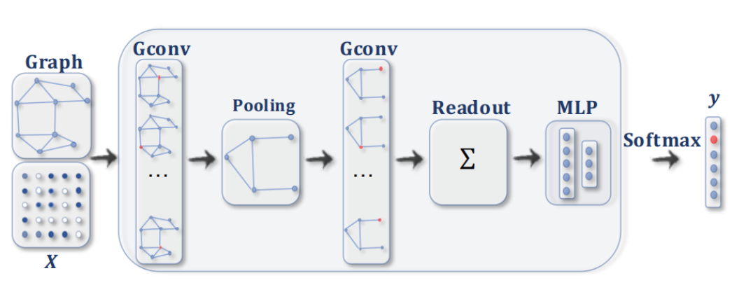
Generic Architecture
A GNN boils down to:
Convolution (local dependencies)
Local Pooling (reduce dimension)
Global Pooling (=Readout): transform graph to vector
MLP classification
Graph Convolutional Network
Convolutional filters, similar to CNNs, passed on the graph nodes to update them with respect to their neighbors’s features. Definition:
\[h_i' = \sigma \left( \sum_{j \in \mathcal{N}_i} \frac{1}{\sqrt{|\mathcal{N}_i| |\mathcal{N}_j|}} W h_j \right)\]
-
\(W\): parameters of the layer
-
\(h_i\): features at node \(i\)
-
\(\mathcal{N}_i\): neighborhood of node \(i\)
Graph Attention Networks
Aggregating features from its neighbors, weighted by attention coefficients. Definition:
\[h'_i = \sigma\left(\sum_{j \in \mathcal{N}_i} \alpha_{ij} \mathbf{W}h_j\right)\] \(\alpha_{ij}\) : attention coefficient indicating the importance of node \(j\)’s features to node \(i\) \[\alpha_{ij} = \frac{\exp\left(\text{LeakyReLU}\left(\mathbf{a}^T[\mathbf{W}h_i \| \mathbf{W}h_j]\right)\right)}{\sum_{k \in \mathcal{N}_i} \exp\left(\text{LeakyReLU}\left(\mathbf{a}^T[\mathbf{W}h_i \| \mathbf{W}h_k]\right)\right)}\]
Graph Isomorphism Network Convolution
Maximize the representational/discriminative power of a GNN. Definition:
\[
\mathbf{h}^{\prime}_i = \text{MLP} \left( (1 + \epsilon) \cdot
\mathbf{h}_i + \sum_{j \in \mathcal{N}_i} \mathbf{h}_j \right)
\] \(\epsilon\) : learnable parameter or a fixed scalar
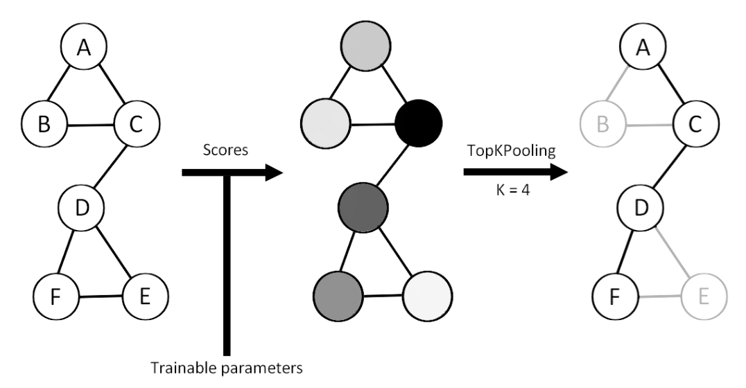
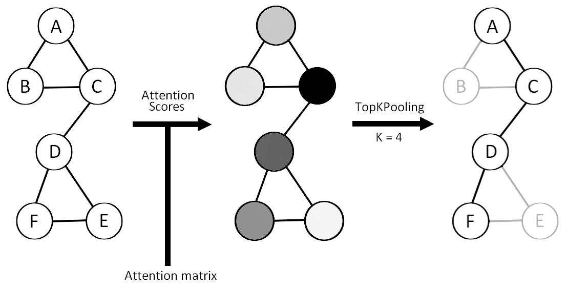
Top-K pooling operator
Top-K Pooling retains only the top-K nodes with the highest scores.
Self-Attention Graph Pooling
Top-K Pooling with attention scores.
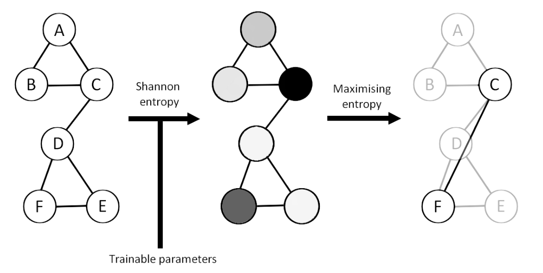
MEWIS Pool (Maximum Entropy Weighted Independent Set Pooling)
Maximizing the Shannon Entropy
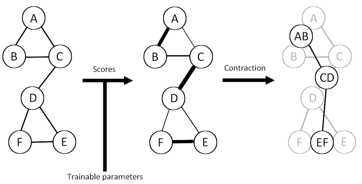
EDGE pooling
Pairing nodes based on scores.
Our datasets
|
|
MUTAG
|
PROTEINS
|
ENZYMES
|
NCI1
|
|
Number of graphs
|
188
|
1113
|
600
|
4110
|
|
Number of classes
|
2
|
2
|
6
|
2
|
|
Number of features
|
7
|
3
|
3
|
37
|
|
Homophily
|
0.721
|
0.657
|
0.667
|
0.631
|
Mean vs Max Readout
Test the differences with Wilcoxon tests.
|
|
p-value
|
Mean difference
|
Best architecture
|
|
MUTAG
|
0.258
|
-0.008
|
GINConv_EDGE_max
|
|
PROTEINS
|
0.33
|
0.009
|
GCN_EDGE_max
|
|
ENZYMES
|
0.207
|
-0.01
|
GINConv_EDGE_mean
|
Result
Since p-value > 0.05, the results are equivalent between mean and max readout. \(\hookrightarrow\) We will only keep the global max pooling
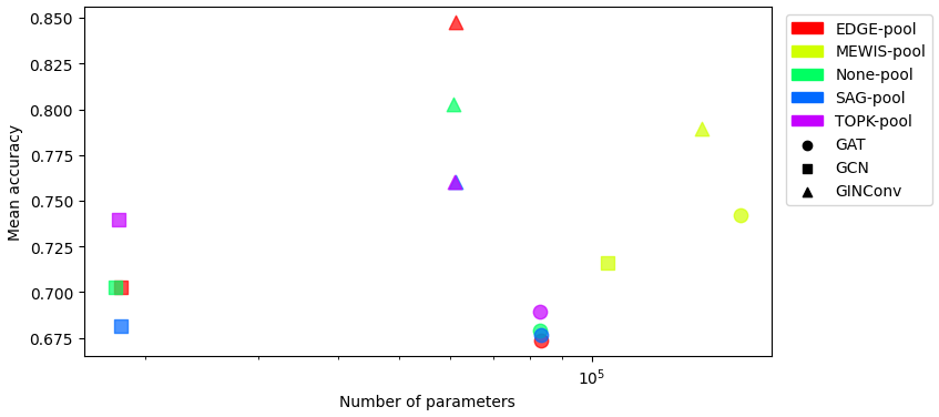
Test accuracy vs Number of parameters on MUTAG
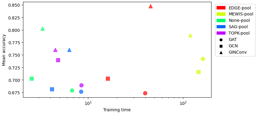
Test accuracy vs Train
time on MUTAG
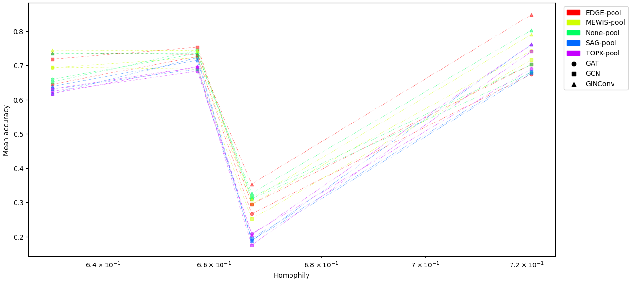
Test accuracy vs Homophily
Results by pooling
|
|
|
ENZYMES
|
MUTAG
|
NCI1
|
PROTEINS
|
Train time
|
|
EDGE
|
GCN
|
0.294 ± 0.026
|
0.703 ± 0.081
|
0.717 ± 0.015
|
0.753 ± 0.024
|
1327
|
|
GIN
|
0.353 ± 0.039
|
0.847 ± 0.063
|
0.735 ± 0.010
|
0.731 ± 0.017
|
1156
|
|
MEWIS
|
GIN
|
0.309 ± 0.055
|
0.789 ± 0.077
|
0.744 ± 0.006
|
0.743 ± 0.016
|
4365
|
|
None
|
GCN
|
0.316 ± 0.044
|
0.703 ± 0.065
|
0.651 ± 0.015
|
0.743 ± 0.029
|
40
|
|
GIN
|
0.327 ± 0.042
|
0.803 ± 0.068
|
0.734 ± 0.018
|
0.733 ± 0.028
|
59
|
|
SAG
|
GAT
|
0.189 ± 0.025
|
0.676 ± 0.062
|
0.617 ± 0.024
|
0.722 ± 0.050
|
112
|
|
GCN
|
0.195 ± 0.033
|
0.682 ± 0.073
|
0.630 ± 0.021
|
0.689 ± 0.041
|
53
|
|
GIN
|
0.188 ± 0.040
|
0.761 ± 0.081
|
0.639 ± 0.036
|
0.714 ± 0.039
|
59
|
|
TOPK
|
GAT
|
0.208 ± 0.054
|
0.689 ± 0.093
|
0.623 ± 0.045
|
0.682 ± 0.033
|
110
|
|
GCN
|
0.176 ± 0.035
|
0.739 ± 0.075
|
0.631 ± 0.034
|
0.694 ± 0.032
|
55
|
|
GIN
|
0.205 ± 0.056
|
0.761 ± 0.079
|
0.617 ± 0.033
|
0.697 ± 0.027
|
56
|
Best architecture per pooling:
|
Dataset
|
ENZYMES
|
MUTAG
|
NCI1
|
PROTEINS
|
|
EDGE
|
GIN
|
GIN
|
GIN
|
GCN
|
|
MEWIS
|
GIN
|
GIN
|
GIN
|
GIN
|
|
None
|
GIN
|
GIN
|
GIN
|
GCN
|
|
SAG
|
GCN
|
GIN
|
GIN
|
GAT
|
|
TOPK
|
GAT
|
GIN
|
GCN
|
GIN
|
Results by architecture
| GAT |
MEWIS |
\(0.295 \pm0.040\) |
\(0.742 \pm0.086\) |
\(0.693 \pm0.008\) |
\(0.722 \pm0.022\) |
3225 |
|
None |
\(0.310 \pm0.053\) |
\(0.679 \pm0.087\) |
\(0.659 \pm0.023\) |
\(0.734 \pm0.027\) |
90 |
| GCN |
EDGE |
\(0.294 \pm0.026\) |
\(0.703 \pm0.081\) |
\(0.717 \pm0.015\) |
\(0.753 \pm0.024\) |
1327 |
|
None |
\(0.316 \pm0.044\) |
\(0.703 \pm0.065\) |
\(0.651 \pm0.015\) |
\(0.743 \pm0.029\) |
40 |
|
TOPK |
\(0.176 \pm0.035\) |
\(0.739 \pm0.075\) |
\(0.631 \pm0.034\) |
\(0.694 \pm0.032\) |
55 |
| GIN |
EDGE |
\(0.353 \pm0.039\) |
\(0.847 \pm0.063\) |
\(0.735 \pm0.010\) |
\(0.731 \pm0.017\) |
1156 |
|
MEWIS |
\(0.309 \pm0.055\) |
\(0.789 \pm0.077\) |
\(0.744 \pm0.006\) |
\(0.743 \pm0.016\) |
4365 |
Best pooling per architecture :
| GAT |
None |
MEWIS |
MEWIS |
None |
| GCN |
None |
TOPK |
EDGE |
EDGE |
| GIN |
EDGE |
EDGE |
MEWIS |
MEWIS |
Conclusion
Key idea
- GNN/CNN : convolution / pooling
- Best pairing : GINConv - Edge / Mewis pool
- Attention : dataset / architecture
Work to be done
- Bigger datasets
- Tuning the architecture
- Other methods